Optical Flow
By Žan Pušenjak
Advanced Computer Vision Methods, FRI, University of Ljubljana
computer-vision
Introduction
In this exercise, we were given the task of computing the optical flow in a sequence of images. We compared different computational approaches using different methods and their improvements. We looked at how the algorithms act when ran with different parameters and selected the best ones.
Experiments
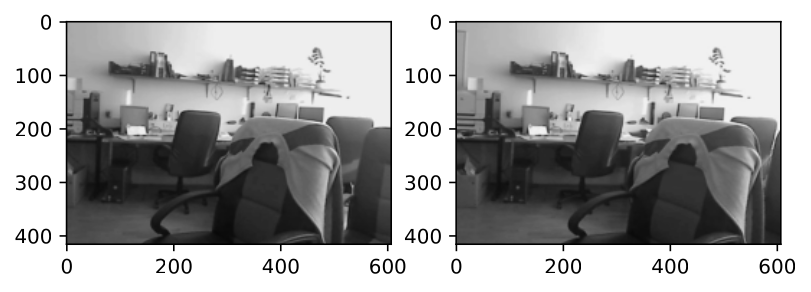
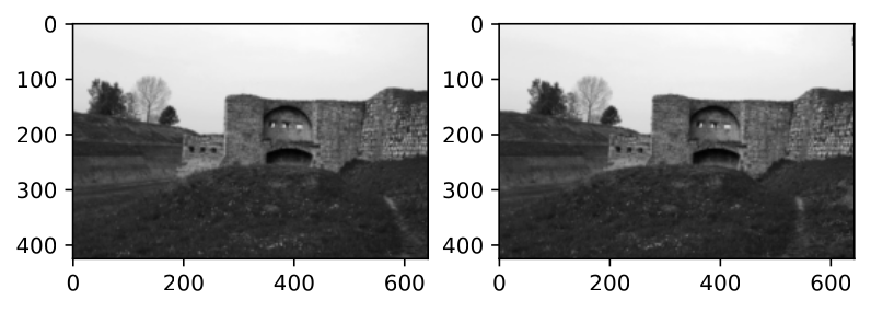
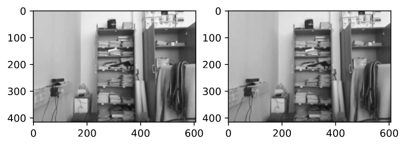
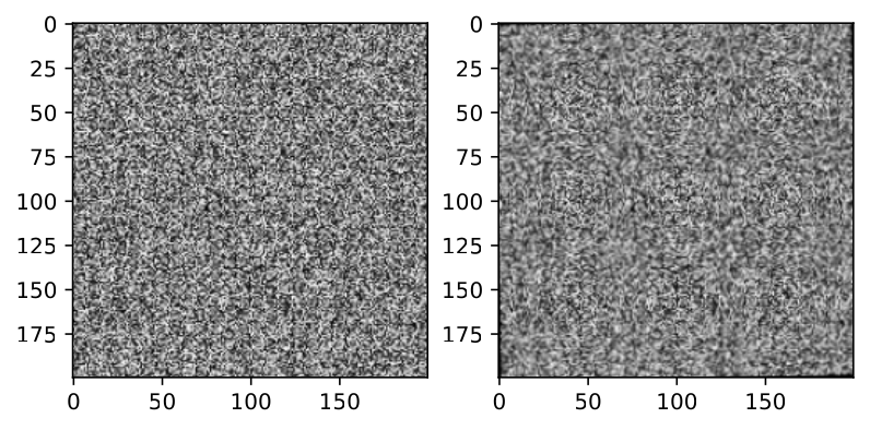
We implemented two algorithms. Lukas-Kanade (LK) and Horn-Schnuck (HS) optical flows. To further improve the speed and results we improved LK with the pyramidal approach and pre-initialized HS with the LK method. We computed the optical flow (OF) on a random noise rotated by one degree and three pairs of images. Pairs can be seen on Figure 5 and will be referenced throughout the report.
Lukas-Kanade
LK algorithm depends on two variables. that denotes the size of the neighborhood for computing the flow at each pixel and that is used in gaussian smoothing and derivation. We fixed since it gave the best results in general, but the variation in did not change the results that drastically. On the other hand does have a different effect based on the image size. Taking that into account we set the parameter dynamically with the formula where and are the width and height of the image. This gave us an algorithm that worked on different sizes of images out of the box with no parameter tweaking.
The results on all the test images can be seen on Figure 10
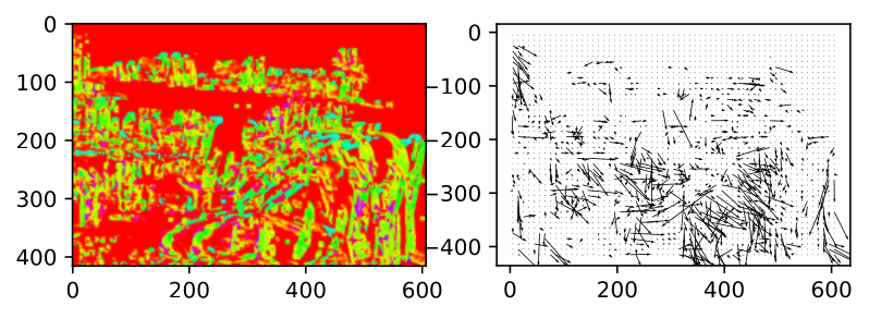
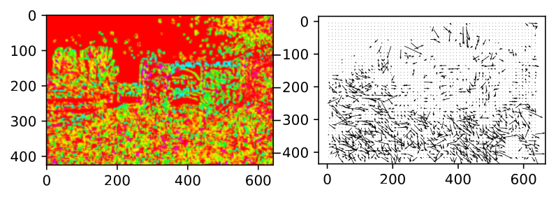
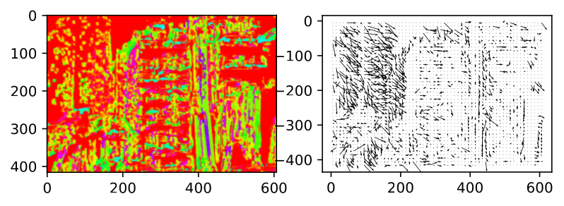
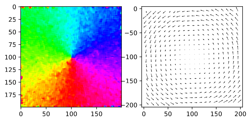
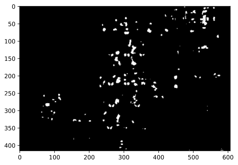
Because of our assumptions while deriving the OF this LK method is not stably in areas with similar texture. That is why we used Harris corner detection1 method to show the areas where the algorithm is stable (an example of the stability regions on image 3 can be seen on Figure 11, where the unstable regions are black).
Pyramidal Lukas-Kanade
To improve the classic LK algorithm we used the pyramidal approach that can detect larger movements on the flow. We observed that when building full pyramids some monotone images, like the rotating random noise would get a worse OF computation. This happened, because the very top of the pyramid that detects the large movements should not detect a movement, but because the noise is similar throughout there is a chance that a movement will be detected. To avoid that we limited pyramid build process to not go further if the image at current level is not at least pixels.
The results on all the test images can be seen on Figure 16
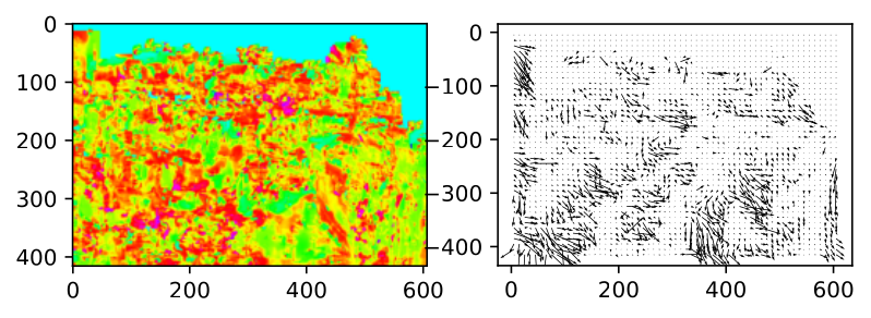
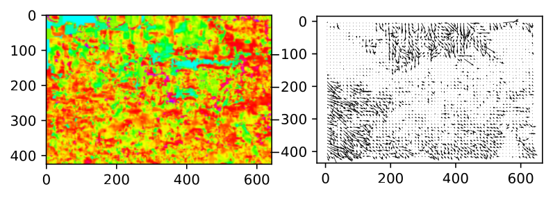
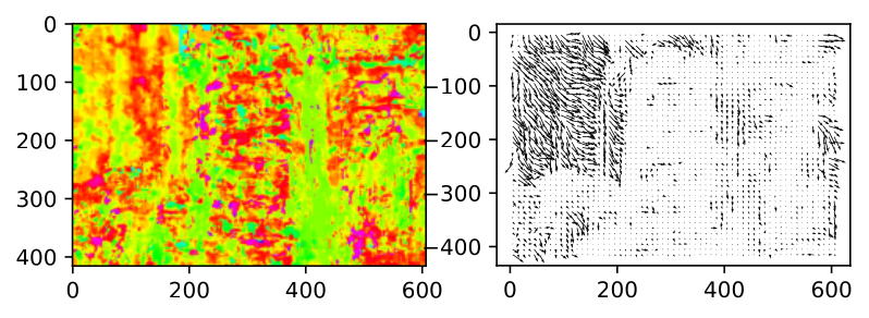
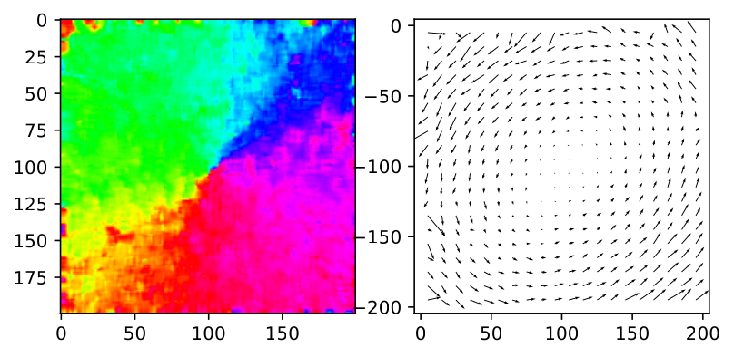
When comparing results with the normal LK we can observe that this approach gives better results that are much less noisy and work better when the depths of objects vary.
Horn-Shnuck
With the HS algorithm there are more parameters to be determined, prior to the computation. Similarly as with LK we used gauss smoothing and derivation so we determined and the same way as with LK. Since HS is a iterative algorithm it needs a stopping scenario. We determine that with parameters that represents the maximum number of iterations and that represents the threshold for change. If the change in current iteration is too small the algorithm will stop. With experimentation we decided on the values and Additionally HS has a parameter that determines the trade-off between smoothness and accuracy of the OF. Since each image has a different optimal we fixed its value to and gave the user an option of controlling the parameter. It would be interesting to find a way to find the optimal lambda value by using a metric to describe the accuracy of the computed OF and a method like grid search or to set the parameter based on the images properties (texture complexity, noise level...).
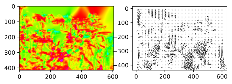
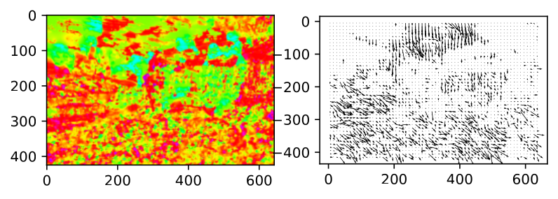
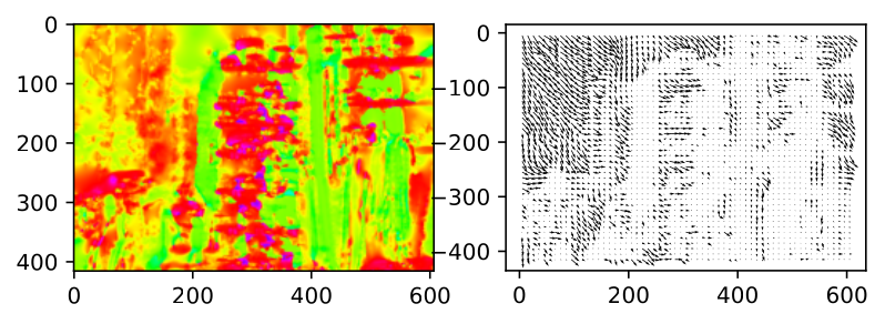
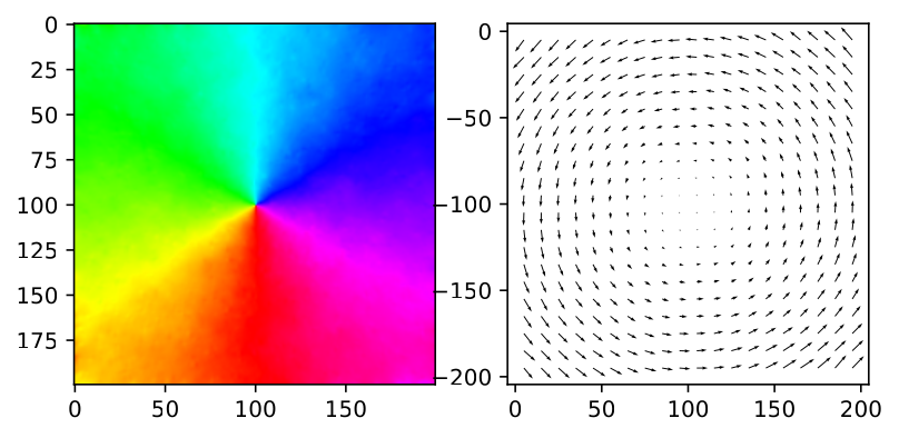
The results on all the test images can be seen on Figure 21
Preinitialized Horm-Shnuck
HS algorithm takes much longer to compute than LK due to its iteration based nature. To battle that we tried to first compute the OF with LK and than ran the HS computation of the output of LK hoping for improved speed and maybe even improved results. In Table 1 we can observe that the time did not improve drastically and the results stayed the same.
| 1-5 Algorithm | LH | LK pyramid | HS | HS initialized |
|---|---|---|---|---|
| Time | 0.02 | 0.04 | 11.02 | 10.49 |
Conclusion
When comparing the final results we can see that the LK-pyramidal and HS gave very similar results (although LK-pyramidal was noisier with larger variance), while the normal LK gave a very noisy OF compared to the previous two and only worked perfectly on the rotated random noise. We can observe that normal LK had difficulty with depth, as the perception of movement changes with depth and the algorithm does not account for that.
https://docs.opencv.org/4.x/dc/d0d/tutorial_py_features_harris.html↩︎