Model Evaluation

By Žan Pušenjak

Machine Learning for Data Science, FRI, University of Ljubljana

Mar 23, 2025
machine-learning model-evaluation

Models and data

We used four different models on a single dataset and evaluated their performances.

Data

We used data about basketball shots having six categorical features: (1) ShotType (target feature), (2) Competition, (3) PlayerType, (4) Transition, (5) TwoLegged, (6) Movement

and two numerical features: (7) Angle and (8) Distance. The dataset consisted of 5024 entries. We assumed that the data was optimal with no outliers or false values.

In Table 1 we can see the frequency and the number of occurrences of each type of shot in the data.

*ShotType* occurrences and frequency.
1-3 ShotType	Occurrences	Frequency
above head	3055	0.608
layup	973	0.194
other	439	0.087
hook shot	397	0.079
dunk	99	0.020
tip-in	61	0.012

Models

The predictions were made using the following models.

Baseline classifier (The predictions were equal to the relative frequencies of the classes in the training set.)
Logistic regression
KNN (We used two approaches to find the optimal parameters.)
1. Training fold performance optimization
2. Nested cross validation

Evaluation

For the evaluation metrics we chose Accuracy and Log Loss. We used ten fold Cross-validation to compute the final estimated metrics and their uncertainties.

KNN parameter optimization

Finding the best parameter $k$ for the KNN model was done in two ways that counted as two different models in the final evaluation.

Training fold performance optimization
We tested all possible values for $k$ while training and predicting on only the train set. Than we used the best $k$ to predict the test set
Nested cross validation
Using another Cross-validation on the train set we firstly found the best $k$ and ten trained the model on full train set with selected parameter $k$ and predicted the test set

Because testing for every $k$ would be computationally expensive, we limited ourselves to a selected set of possible values. We chose $k \in \{10,20,30,40,50,60,70,80,90,100\}$ We could further improve the results by repeatedly changing the set to arrive at the actual optimal value.

Data correction

Later we acquired additional information about the data generating process. The relative frequencies of Competition types were not correctly represented in the dataset. The true frequencies ( $fq_{class}$ ) were $0.6$ for NBA and $0.1$ for the rest of the types. Taking this new knowledge into account, we recomputed the evaluations and compared them with original values.

We corrected the data by changing the class weights to $w_i = fq_{class} * \frac{N_{class}}{N}$ where $N_{class}$ is the number of samples form that class and $N$ is the number of all samples, and normalizing the weights.

Results

The results for the original and corrected data can be observed in Table 2 and Table 3.

Estimated model performance on original data.
1-3 Model	Accuracy	Log Loss
Baseline	0.6081 $\pm$ 0.0068	1.1658 $\pm$ 0.0132
Log. reg.	0.7352 $\pm$ 0.0062	0.6677 $\pm$ 0.0128
KNN	0.7040 $\pm$ 0.0064	2.3461 $\pm$ 0.1066
KNN (nested)	0.7040 $\pm$ 0.0064	2.3461 $\pm$ 0.1066

Estimated model performance on corrected data.
1-3 Model	Accuracy	Log Loss
Baseline	0.6081 $\pm$ 0.0068	1.1480 $\pm$ 0.0128
Log. reg.	0.7531 $\pm$ 0.0060	0.6639 $\pm$ 0.0127
KNN	0.7073 $\pm$ 0.0064	2.3794 $\pm$ 0.1075
KNN (nested)	0.7073 $\pm$ 0.0064	2.3794 $\pm$ 0.1075

Logistic regression achieved the best results. Although the KNN models achieved only a slightly worse Accuracy their Log loss was the highest, even higher than that of the Base classifier. We explained that with the properties of the models predictions. Since KNN generates more strict prediction probability and Log loss penalizes low true class probabilities exponentially the loss will naturally be high if the model does not fit the data almost perfectly.

We also observed that both KNN models achieved the same scores, meaning that both methods selected the same parameter $k$ as the optimal one.

Looking at the results on the corrected data we can see that the correction did not change the scores drastically. Logistic regression saw an improvement in the accuracy while the other scores did not change enough to attribute a high importance to the correction. We explained that with the argument that players in all competitions make the shots similarly (above head - both feet on the ground, dunk - movement is present...) so adjusting the importance of a particular competition is not a crucial fix.

Error dependence

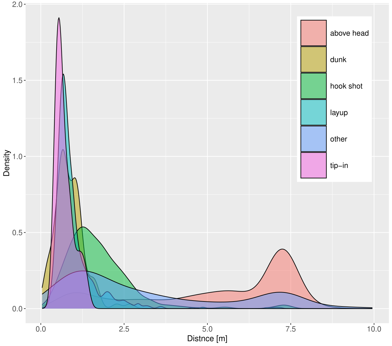
Distribution of *ShotType* with respect to *Distance* feature.

Using domain knowledge we suspected that the Distance feature determines the ShotType heavily, since shots like layup, tip-in or dunk can only be performed with a small distance so when the distance grows there are less options for the type of shot a player can make. Plotting the distributions of all types on Plot 1 we can clearly see the differences. At a longer distance the only viable shot type is almost exclusively above head while at the one to two meter distance its density reduces heavily and types like dunk or layup distributions’ spike.

Further plotting the dependence between the Distance and Log loss (Plot 2) we can see that the loss diminishes significantly after Distance reaches values greater than four meters. An unexpected increase in loss happens at seven meters. Looking back at Plot 1 we see that that is where the peak of above head shot type distribution lies and the other shot type density increases as well, hence the increase in loss can be attributed to that.

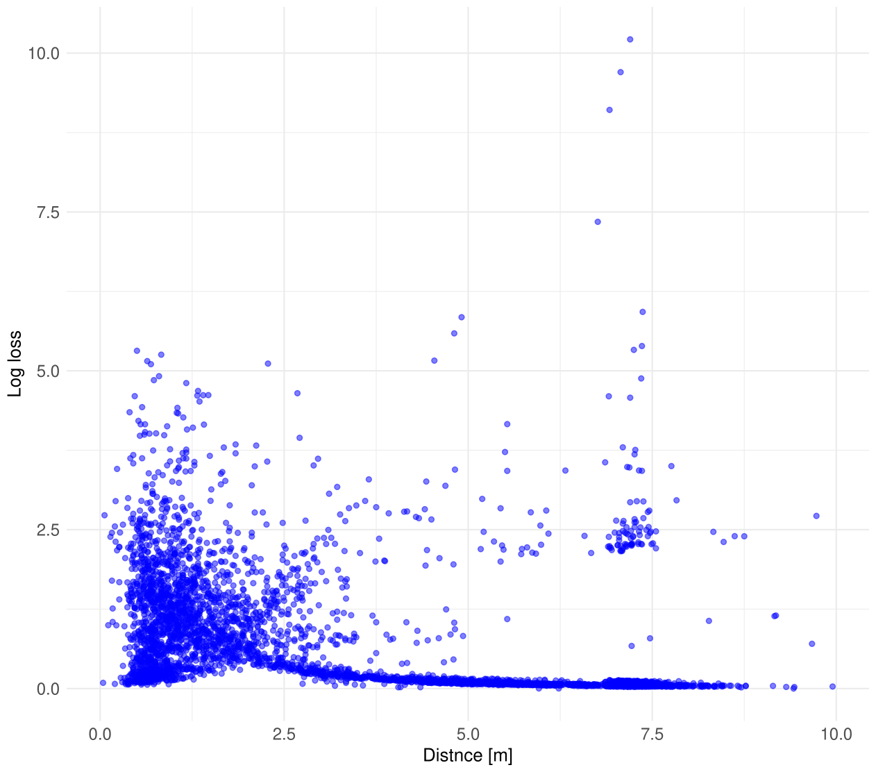
Example of an binarized image after zero crossing detection.

Since the distributions of shot types differ so drastically when the distance is small versus when it is large it would be interesting to train two different models, one for shots closer than four meters and one for shots made further away. Additionally since the other shot type represents quite a large portion of the data (1̃0%) it would be useful to dedicate additional time to classify those entries or discard them as noise.