Kernel Methods
By Žan Pušenjak
Machine Learning for Data Science, FRI, University of Ljubljana
machine-learning
Implementation
We implemented the kernelized ridge regression (KRR) and Support Vector Regression (SVR). To go along with the models we implemented three different kernels:
Polynomial kernel
RBF kernel
Linear kernel
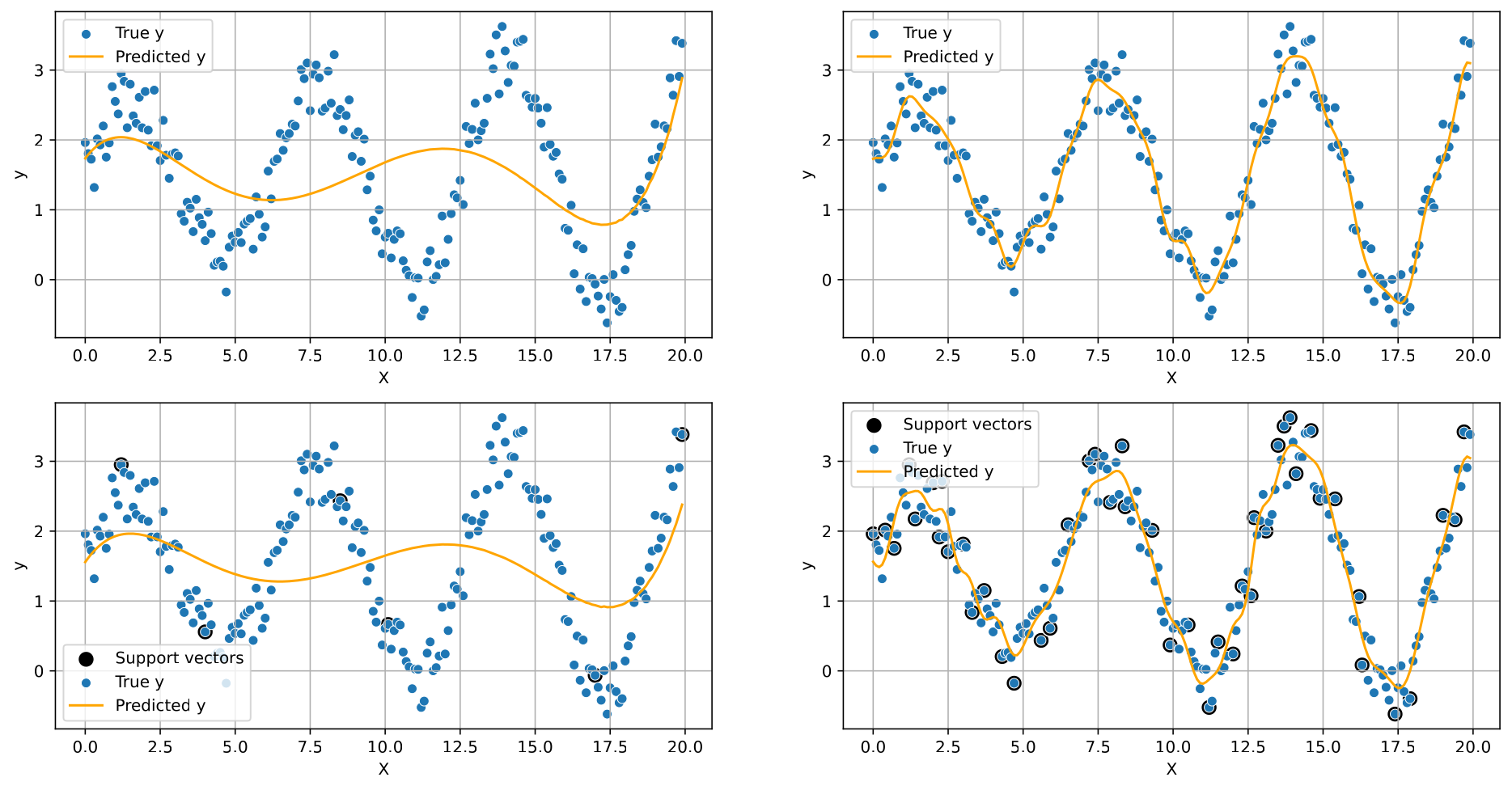
We used the implementations on sine data. We could observe that the choice of the parameters greatly affected the fit. With SVR we had to be careful to manage the number of support vectors. We used parameters in Table1 and were able to achieve results seen on Figure6
| 1-4 Model | Kernel | Parameters | |
|---|---|---|---|
| KRR | |||
| RBF | |||
| KRR | |||
| Polynomial | |||
| SVR | |||
| RBF | |||
| SVR | |||
| Polynomial | |||
Where is the degree of the polynomial and is the coefficient in the polynomial.
We observed that the RBF kernel achieved an excellent
fit to the data, while the Polynomial kernel struggled to
capture the underlying pattern effectively.
Fitting the housing data
We trained our model to fit the housing data. The combinations of the
kernels and methods stayed the same, but this time we used
nested-cross-validation (NCV) to determine the best
parameter
.
We also fixed
and compared the two results. To determine the
parameter for SVR, we made tried to fit the model on some samples and
looked at the number of the support vectors. Observing the
results in 2 we can see that the parameter did not
change the number so we fixed it at
| MSE | Support Vectors | |||
|---|---|---|---|---|
| 0.1 | 26.53 | 12.05 | 95.89 | 28.47 |
| 0.3 | 26.47 | 12.05 | 91.42 | 28.44 |
| 0.5 | 26.43 | 12.07 | 96.17 | 24.60 |
| 0.7 | 26.34 | 12.03 | 98.69 | 25.83 |
| 0.9 | 26.26 | 12.01 | 101.30 | 23.25 |
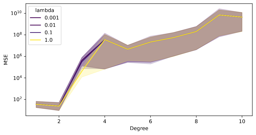
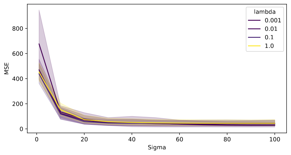
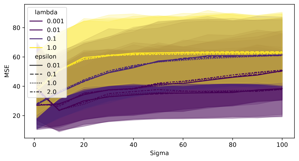
Because computation of lots of parameter values was not possible we evaluated the models with a simple train-test split to get a feel for what values of parameters to explore more deeply. The results can be observed on Figure 1 for KRR and Figure 2 for SVR.
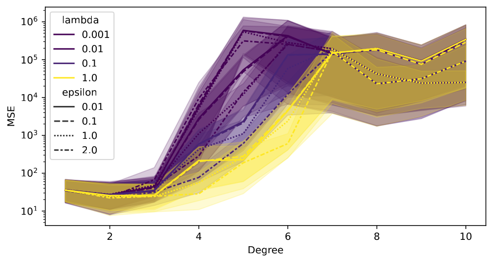
Thanks to this simple exploration we were able to confidently chose
parameters
,
and
.
We started with leave-one-out NCV but because of
computational reasons we abandoned that approach and used a
10-fold NCV.
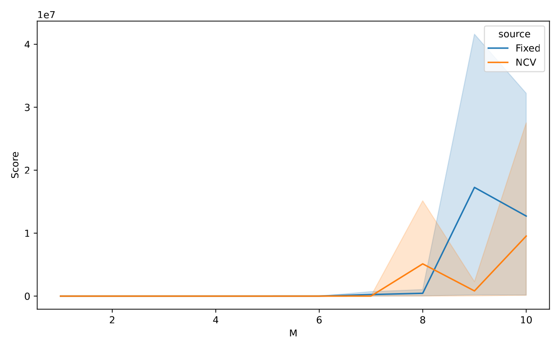
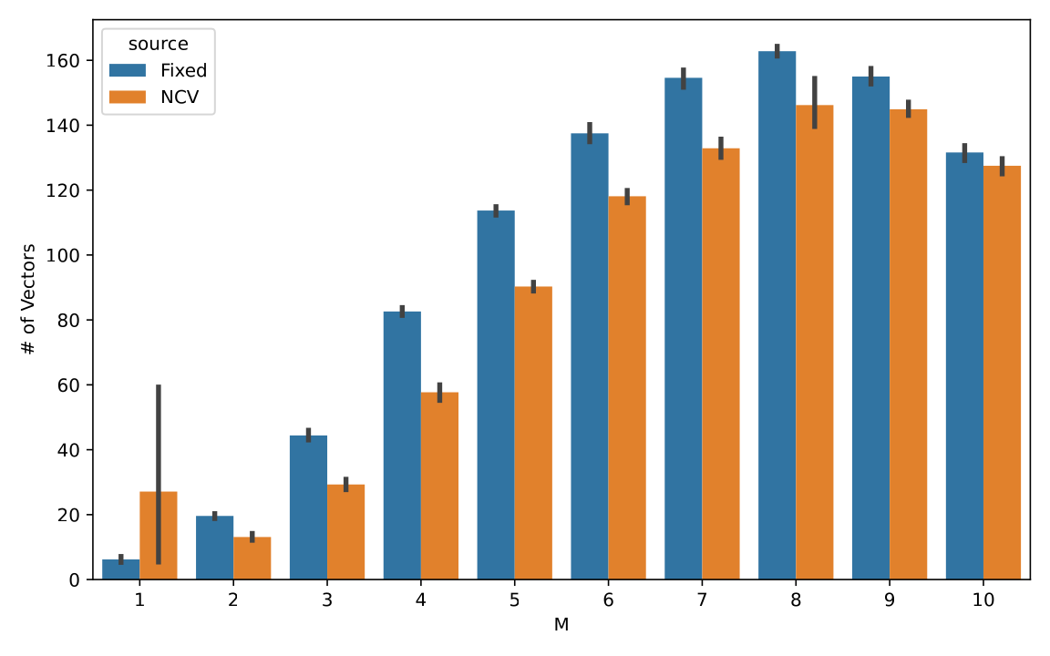
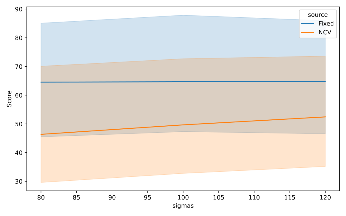
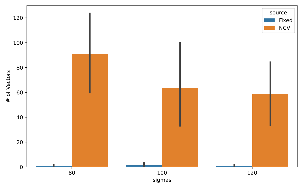
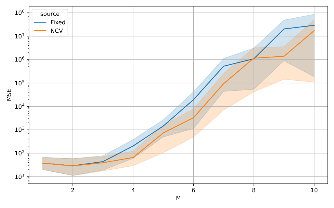
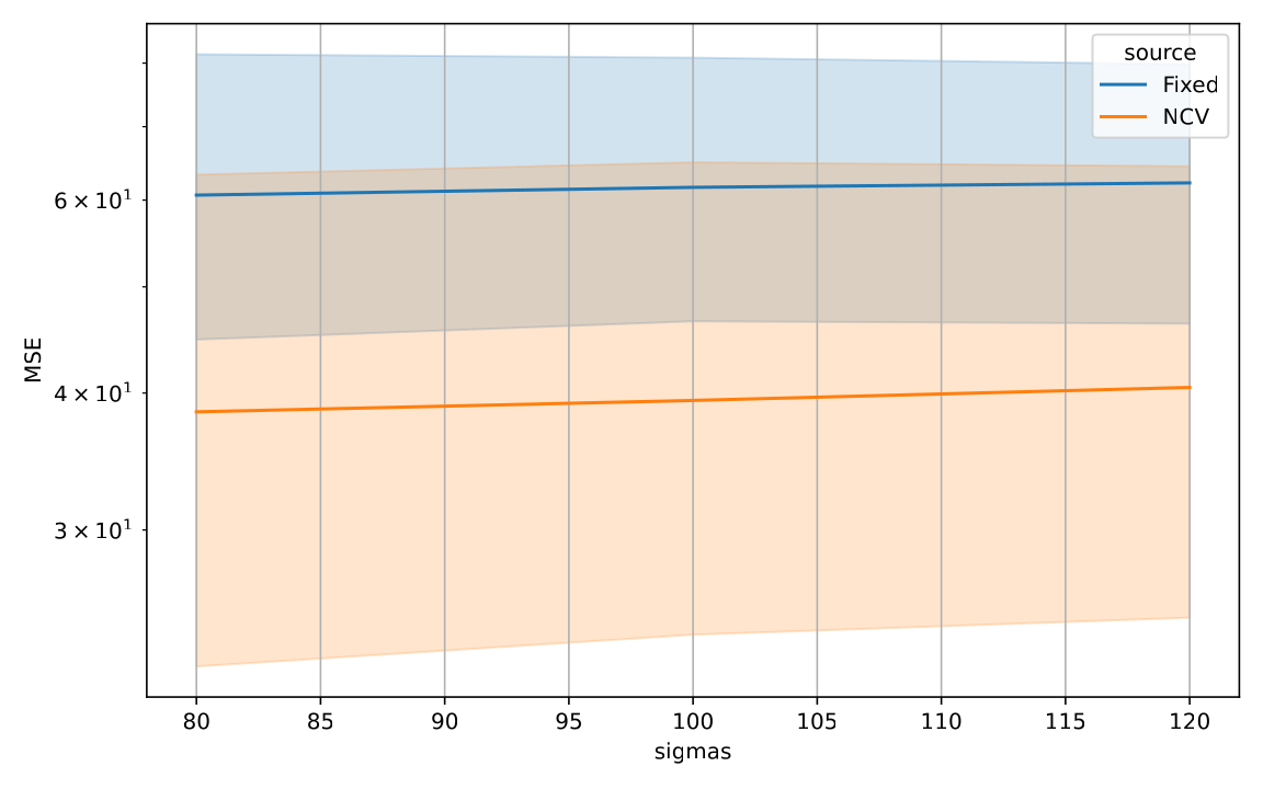
The results can be observed on Figures 3, 4 and 5. We can see that the NCV approach outperforms the fixed model, and would likely perform even better if we could check even more values for . We can see that with polynomial kernel, the number of support vectors increases as the degree increases where with RBF kernel the sigmas do not have any effect, but the fixed lambda yields less vectors.