Generalized Linear Models
By Žan Pušenjak
Machine Learning for Data Science, FRI, University of Ljubljana
machine-learning
Implementation
We implemented both models by minimizing their log-likelihood with the help of the function 1.
To achieve accurate interpretability, we used the first class as reference class. With that we achieved the right number of parameters to optimize:
Multinomial
Ordinal
Where is the number of classes and is the number of features.
Application of the Multinomial Regression
We used the provided data set of basketball shot types2 and our model implementation to provide some insight into the relationship between the ShotType feature and other features.
We additionally prepared the data by one hot encoding the categorical features Competition, PlayerType and Movement and normalizing the numerical features Distance and Angle. Finally we removed highly correlated features (features with correlation coefficient ), which allowed us to better interpret the final parameters.
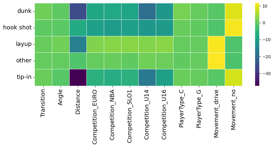
We used the parameter matrix as the main instrument for our findings. A parameter represents the log-odds of observing the class as opposed to observing the reference class. So a higher value will increase those odds for the class and a lower value will decrease them. Our reference class was above-head
Observing Figure 1 we selected the highest and lowest and tried to find any explainable relations.
Competition U14
We can observe that two parameters for the Competition_U14 feature are negative, values being:
dunk:
tip-in:
So if the shot was recorded in a U14 basketball game the chances of observing a dunk or a tip-in rather than an above-head shot are significantly decreased. This is a logical explanation since the players at that age are usually not tall enough to perform a shot of that type and mostly throw above-head.
Movement
The Movement_drive and Movement_no features positively influence the hook-shot, layup and other types, with the exact parameter values being:
for Movement_drive
layup:
other:
for Movement_no
dunk:
hook-shot:
tip-in:
This tells us that the chances of observing a layup or other shot type instead of above-head will increase if there is drive movement present. The unexpected results that we could not interpret were that if there is no movement present a dunk, hook-shot or tip-in will occur more regularly.
On the other hand
Distance
It is apparent the Distance feature was the most important feature on some classes. This is expected, as the further the player is from the rim, the less likely he is to perform a tip-in, dunk or layup, in that order, and that reflects on the parameters.
tip-in:
dunk:
layup:
Application of the Ordinal Regression
We made some synthetic data using a data generating process (DGP) of ordinal value to show that the ordinal regression model will outperform the normal multinomial regression with suck DGP. We used accuracy as the metric for comparison. The performance of the models can be observed on Figure 2 where we observe that the ordinal regression clearly outperforms the multinomial one. We can also see that increasing the data set does not attribute to the results.
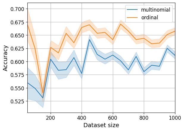
Even when increasing the data set size to the ordinal regression still achieved a better accuracy seen in Table 1.
| 1-2 Model | Accuracy |
|---|---|
| Ordinal reg. | |
| Miltinomial reg. |