Demand Forecasting for a Gulf-Region Furniture Provider
By Anton Križnar, Žan Pušenjak, Matej Vrečar
Faculty of Computer and Information Science, University of Ljubljana
forecasting time-series neural-networks
Introduction
Demand forecasting is a crucial component of data-driven decision-making for retailers, enabling them to optimize their supply chains and operations. This leads to better product offerings combined with shorter delivery times for the final customer. In this project, we were working with In516ht and Alghanim Industries on demand forecasting for a furniture retailer in the Gulf region, Safat Home, with a goal of streamlining the demand prediction process, which is currently estimated by individuals.
Furniture retail
Retailers focus on providing the connection between the producers and the consumers, traditionally through physical stores, but lately additional sales channels (like online stores, affiliate campaigns, etc. ) are being introduced into the business.
The biggest challenge these businesses face is inventory management. If a customer orders a product, that product needs to be in stock, but storage capacity is costly, so the retailers want to keep as little inventory as possible while simultaneously never running out of stock. That is why demand forecasting is a crucial part of retail business strategy. Knowing the amount of demand will allow the business to order additional stock according to the demand forecast.
An additional aspect of the furniture business is product bundles. Most of the time, a product is not sold separately but rather in a bundle that consists of different products, a multiple of the same product, or a combination of both. So if only one product from the bundle is missing, the entire bundle is out of stock, hence, it is even more important for the inventory to be present at all times.
All retail businesses are heavily influenced by external factors such as the state of the economic market, holidays, and even overall seasonality. The latter is the most impactful, especially in the furniture retail sector, and should be taken into account when analyzing the data.
Lastly, if the business is large enough, it features multiple stores and storage facilities, possibly located in different countries with completely separate supply chains, which again alters the demand forecasting process.
Course of the project
Competition partners have realized at the mid-point check-up that their data is too sensitive for us to work on, so they pulled out of the collaboration. For this reason, we have decided to find a dataset in a similar industry to the one we were promised, so the research that we have done remains relevant. We found the M5 competition dataset on Kaggle1, on which the competition on demand forecasting for retail was conducted.
We selected this dataset because it was previously shown to be representative of retail business sales data, compared to retailer time series from Greece and Ecuador (Theodorou et al. 2021).
M5 dataset
For the development of our method, we chose a public dataset from the M5 retail sales forecasting competition, with 3,000 product sales spanning over 5 years, from 29/1/2011 to 22/5/2016 (Makridakis et al. 2022). This dataset was selected because it is large enough to run experiments on and is very representative of our retail business. The provided timeseries are structured in a hierarchy and can be aggregated to obtain different levels of demand. The dataset includes calendar events, sales, and price data from the world’s biggest retailer.
Sales data
The data is a subsample of 30,490 product sales of different department stores of the biggest retailer in the world, Walmart (Makridakis et al. 2022). The dataset consists of sales transactions, prices, and calendar data.
Sales - the main document that describes the sales of the product per day. It includes information about the level in the hierarchy, where the product is situated.
Prices - information about the prices of products for each of the stores on a date.
Calendar - special dates information like holidays, supplemental nutrition assistance program2 (SNAP) activities and other events.
Dataset hierarchy
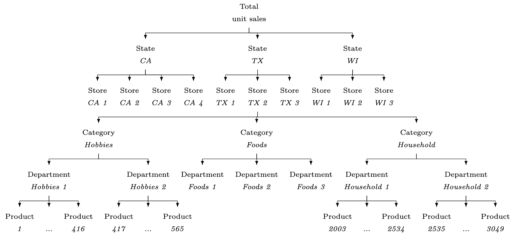
Data is organized in a hierarchy, where 3,049 products are organized in 7 departments of 3 categories Foods, Household, and Hobbies. This sales data of the products is recorded across 10 department stores from 3 states, which can all be aggregated to total unit sales in the data set. This hierarchy in the data is shown in a structured way in Figure 1. With the aggregation of the data on all the different levels, we can further obtain over 42,000 time series. We decided to aggregate the data on the product level, giving us 3,049 time series to work with. Later, we further reduced the number of time series to reduce the computation load.
About the data
Partner company suggested that seasonality is very important in the retail business, so we looked at category-wise aggregation of the data, where a seven-day trend became apparent (Figure 2). Sales throughout the week are very low throughout the week and on Friday, sales start to pick up and reach their peak on Saturday or Sunday. Trends at other intervals do not seem to be as strong, and we noticed that all patterns become more apparent over aggregated data than on the individual product level.
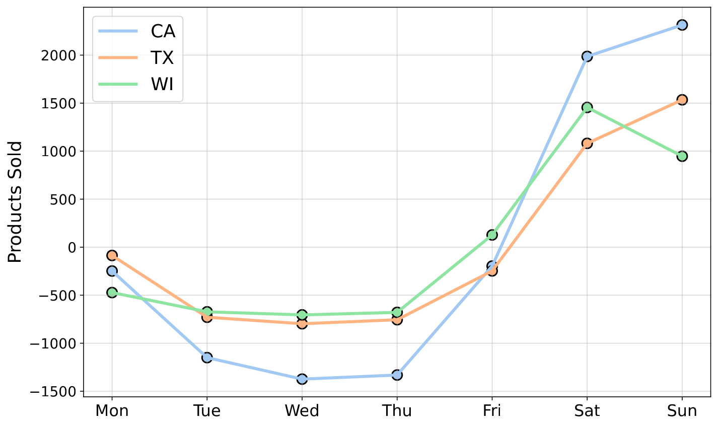
FOODS category sales,
for each of the states.The most sold category in the dataset is foods, followed by the household and hobbies categories. The only apparent event influence is Christmas, where there are no sales on that date every year. The dataset also includes price data through time, but the prices are mostly constant for the vast majority of products.
Data subsample
To reduce the computational load, we decided to select a subsample to speed up data processing. We still wanted to maintain a level of representativeness, but capture the hardest cases in the dataset. The data set includes sporadic time series where a product is not sold for some period of time and then starts selling at some point. These cases could, on one hand, be considered very difficult to predict, but we can avoid a lot of processing this data, because we could employ some different prediction strategy on such cases. Excluding sporadic timeseries also gives us a benefit when evaluating the model, since we could have a period with zero sales, and we could misinterpret the evaluation of the model.
This is why we have selected 101 products among those that have been sold in any 30 days. We sorted such products by the cumulative sum of sales and selected every second product among the top 30 % of the products. This method maintained all categories, and we have lost only 2 departments in the hobbies and household categories. Thus, we have obtained a subsample of data where the errors made by our model will be potentially big, but we still maintained the representativeness of the data hierarchy.
Forecasting methodology
Forecasting has two main approaches, one-step-ahead and multi-step-ahead forecasting. In one-step-ahead, we predict only the next value (Bauer et al. 2019). This type of forecasting is the most common in research. On the other hand, with multi-step, we predict a range of future points together, making it useful for more practical real-world applications. Additionally, multi-step forecasting can be done in two ways. We can make all of the predictions at once, or we can cascade (Linardatos et al. 2024) one-step predictions and then use those predictions to predict even further into the future and repeat that process.
We decided to explore both approaches because we wanted to retain the practical aspect from our original problem while simultaneously working with the dataset in a way that it was used in the competition (one-step-ahead forecasting).
Features
We combined the provided data to construct features:
weekday - the information was one-hot encoded.
day of the month - we encoded the day of the month with sine and cosine to preserve the cyclic nature.
month - the information was one-hot encoded.
event information - event information was provided with the type of the event alongside the category of the event. There could be two events on a single day. We one-hot encoded all of this information.
Since we did not aggregate the products by state, we could not use the SNAP information.
We equipped each data point with historical data for past sales alongside the information about last year’s sales on this day and the day before. This meant that we had to discard one year of data.
Feature selection
To get a better understanding of the data, as well as increase performance, we tried to figure out which features to keep and which ones to throw away. We began by analyzing how much historical data is needed for accurate forecasting. Starting with data from the current day only, we trained a random forest regressor using nested cross-validation and evaluated performance using RMSE. We then progressively included data from one additional previous day at a time, repeating the training and evaluation process up to 14 days in the past. The analysis has shown a significant decline in the error when including the first couple of days, but it appeared to flatline around day 6. We then decided to keep all 14 days of past sales data.
To determine the importance of other features, we initially utilized SHAP3, however, we decided to drop it after the library exhibited random behavior. We therefore decided to follow the same strategy as we did for historical data: training a random forest regressor with past sales data and different subsets of features.
After the analysis, we decided to drop all features connected to events and keep the rest.
Modeling
We tested different models and saw the best results with neural
networks, followed by XGBoost, so we focused on those two in our further
experiments. For the neural network we used two fully connected hidden
layers with 50 and 40 nodes both using the LeakyReLU4 activation functions since the
Sigmoid5 was not modeling the trends
successfully and only ended up learning the average. Both hidden layers
also included a dropout layer with a dropout probability of 10%
Metrics
Our subsample represents 13.10 % of the sales and 8.05 % of the cash flow. To put our method in perspective with real-world application of the retail business, we weighed RMSE results similar to the M5 competition, where we used weighted RMSE (WRMSE) and compared it to the baseline instead of the weighted root mean scaled squared error (WRMSSE). Because we used our own subsample and aggregated them at the product level, we calculated the weights ourselves in the same manner as in the M5 competition (Makridakis et al. 2020). Our version of WRMSE represents how much of the financial loss is caused by inaccurate predictions, based on the following equation:
and is the amount of product sales and is the price.
Weights were computed based on the last 28-day cash flows and represent the ratio of the product’s cash flow and all other cash flows. We compare our approaches to the baseline moving window averaging, which had 37.36 WRMSE. This can be roughly interpreted as how much of the cash flow is lost per prediction, either in terms of lost sales or overstocking.
One-step-ahead neural network
We created a neural network of the type explained above for each of the 101 products. For each, a simple grid search was performed to find the best learning rate parameter. This was automated by utilizing an evaluation set and an early stopping mechanism. For the evaluation of the model, we performed inference 100 times with the dropouts turned on. Then, the mean of the 100 predictions was calculated, and the RMSE was obtained from these. This whole procedure was then completed 100 times, giving us the ability to calculate the mean and standard deviation of the RMSE. We can observe the prediction made by one of these models in Figure 3. It is clear that the model is very successful at identifying the correct trends, but still misses the exact point prediction.
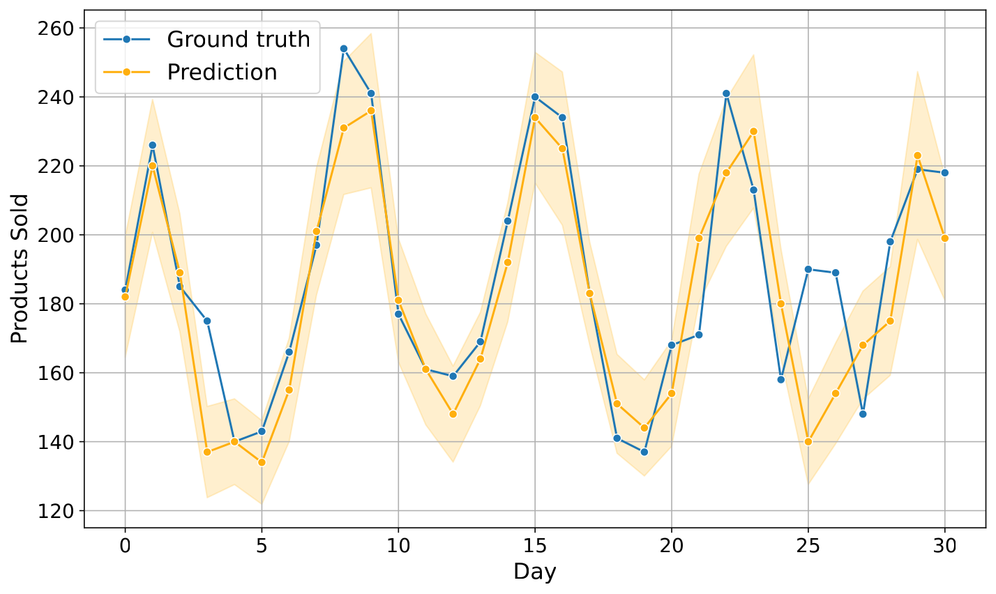
FOODS_3_714 on a period of 31 days. (RMSE: 17.75
0.31.)When evaluating the model, we obtained 17.83 ± 0.21 WRMSE, which is twice as economically efficient as our baseline.
Multi-step-ahead forecasting
To generate multi-step forecasts, we first used a neural network with multiple output nodes, each representing a prediction for a specific day. In parallel, we trained thirty-one separate XGBoost models, with each model dedicated to predicting a specific day in the future. This setup allowed us to directly compare the performance of both approaches when we used the models to forecast thirty-one days ahead for each product. As shown in Figure 4, the neural network generally outperforms the XGBoost models. Additionally, the forecasting error tends to increase linearly with the number of days we are predicting.
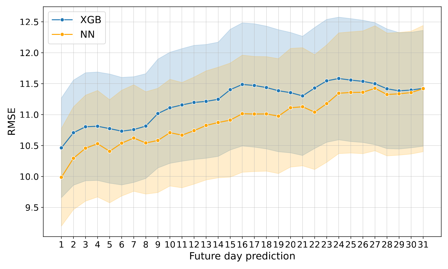
Cascading approach
The cascading multi-step forecasting approach yielded varying results for each of the models. With XGBoost, we saw that the weekly trend showed up, where the predictions for the same weekday the next week are better than for the other weekdays. On the other hand, the neural network model worked similarly, but with some products it scaled out of control and made predictions in the magnitude of , negative predictions, or in some cases even both of those combined. That resulted in a practically infinite error, so using such an approach with a neural network is not feasible.
Compared to the previous approach, this one achieved worse results, so we omitted any further research.
Discussion and Results
Final model performance varied for individual products, where products with high sales numbers were much easier to predict than those with less traffic. Even further, some of the products had higher deviation from the weekly seasonality, and with such cases, the models had more uncertainty and were not able to make as accurate predictions as with the more consistent products.
Predicting multiple days
When it comes to predicting multiple days ahead, we concluded that using a neural network with an output layer sized to match the forecast period yields the most effective results. In practical applications, given that the prediction error increases approximately linearly with the length of the forecast period, we could define an acceptable error threshold and use it to determine the maximum number of days that we can reliably forecast within that limit.
Future work
Since we were computationally limited, it would be interesting to look at the results when predicting the un-aggregated data (meaning each product for each state in each state). With such an aggregation, we could additionally use the SNAP information, which we had to discard in our experiments because of the aggregation.
Discarding the products that had very sparse sales and only keeping the top 101 most sold ones was deemed to be a good idea, but further research could be conducted to find if there exist models and features that could give useful predictions for those products.
Acknowledgments
We thank our mentor, doc. dr. Tomaž Hočevar, for his guidance and support throughout the project. From helping us navigate challenges with external partners to providing steady feedback and warning us about the dead ends, his help was invaluable in helping us advance our work.