Computed Tomography Image Analysis

Introduction

Computed tomography (CT) images are widely used in the medical field. They are used to asses a patients status and non-invasively give the medical analysts an insight into the patients body. The images can often be enhanced via various filtering methods.

It is helpful to develop an algorithm that will detect the edges of different parts of the image and display them for the analysts to faster and better determine the situation.

Methodology

We implemented the Marr-Hildreth edge detector(Marr and Hildreth 1980) in MatLab¹. The algorithm has 3 steps:

1. Convert image to grayscale

2. Filter the image with Laplacian of Gaussian filter

3. Detect zero crossings

We tested the algorithm on four CT images of different body parts.

Zero crossing detection

To detect the edges we look at the zero crossings of the filtered image. Fore each pixel of the filtered image we look at its 3x3 neighborhood. If the two opposing pixels have a different sign that we mark that pixel as an edge pixel. We look in four directions: left to right, top to bottom and both diagonals.

Because some noise is still present we introduce a threshold. Now in addition to opposite signs the absolute value of the difference of the values of the opposing pixels must be greater then the threshold for a pixel to be considered an edge pixel. We again look at the same four directions.

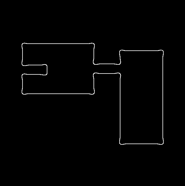
The result of the zero crossing detection is a binarized image with edge pixels having value 1 and other value 0 like seen on Figure 1.

Results

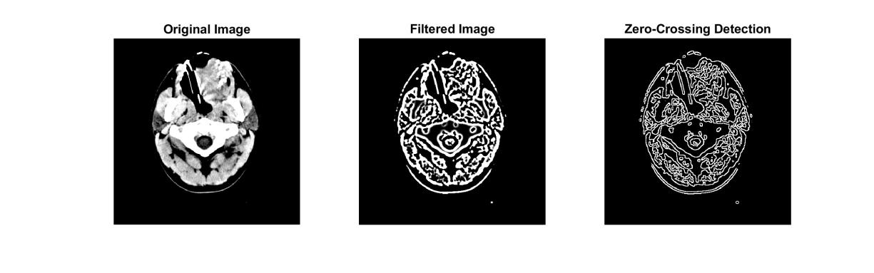
In the Figure 2 we can see a visualization of the algorithm working. The LoG filtering of the image does most of the heavy lifting for us since it already highlights the regions.

Instead of manually setting the parameters for each of the images to find the best ones we decided to calculate them dynamically based on the input image’s properties.

We set $sigma$ to 0.5 percent of the lesser dimension of the image. Then we calculated the size of the kernel as the ceiling of $sigma$ multiplied by 6. Because the kernel must be of odd size, we handeld even sizes by simply adding one. $$kSize' = \lceil 6\sigma \rceil$$ $$kSize = \begin{cases} kSize' + 1, & \text{if $kSize'$ is even} \\ kSize', & \text{if $kSize'$ is odd} \end{cases}$$

To determine the threshold we used MathLab’s graythresh() which implements Otsu’s method(Otsu 1979) for providing the threshold. The method provides the threshold by minimizing the variance within foreground and background pixel groups while maximizing the variance between them. It works by analyzing the image histogram to find the threshold that best separates the two pixel intensity distributions.

Conclusion

The results show the algorithm working and the dynamic calculation of the parameters ensures that the algorithm works on each image as intended and does not require additional finetuning for different images.

If we compare this algorithm to an algorithm like the Canny edge detector we can observe that our edges are multiple pixels wide, so a possible improvement would be to add an additional final step that would thin out the edges like using erosion with a 3x3 kernel or something similar.