Bayesian Time Series

By Žan Pušenjak

Bayesian Statistics, FRI, University of Ljubljana

Jan 18, 2026
bayesian-statistics time-series

Introduction

We were tasked to analyze the measurements of the concentration of nitrogen dioxide (NO2) in the air measured from 1997 to a couple of days ago¹. The goal was to use different time series models to create an ensamble of models weighted with Akaike weights.

The concentration of NO2 in the air is tracked to protect public health and to gauge whether emission reduction policies are working, since the same sources drive both air pollution and greenhouse gases.

Modeling

Data preparation

Since the data was sampled daily we first had to number the rows from 1 to 10373. We denoted this as t. We additionally standardized t with $(x - \mu_x){\sigma_x}^{-1}$ .

Model selection

We used three different time series bayesian models that each built on top of the previous one. Since the data was not stationary we used a Harmonic regression model to remove the trend and seasonality. Next we modeled the remaining noise with a Autoregressive model (AR) and ARMA than compared all three to get the best performing one and built an ensamble for predicting the NO2 values in the future.

Harmonic regression

We set the $\omega$ parameter that denotes the frequency of seasonality by using Fast Fourier transformation and found a high frequency at value $0.1428$ . Because our data is sampled daily we know that $\frac{1}{M} = 0.1428$ so $M=7$ , which signals a weekly seasonality. We calculated $\omega = \dfrac{{2\pi}}{M}$ .

We fitted a harmonic regression model to our data with $\omega$ this value. Note that we used a quadratic trend since it was a much better fit than any other order polynomials. $\begin{aligned} y_t &\mid \alpha, \beta_1, \beta_2, \beta_{\cos}, \beta_{\sin}, \omega, \sigma \sim \mathcal{N}(t_t + s_t, \sigma), \\ t_t &= \alpha + \beta_1 t +\beta_2 t^2, \\ s_t &= \beta_{\cos} \cos(\omega t) + \beta_{\sin} \sin(\omega t). \end{aligned}$

With trend and seasonality removed we used AR and ARMA to model the remainder since it is now a stationary time series.

Autoregressive model

We combined the harmonic regression and AR model. The model took in a parameter $p$ that is a vector of lags, so we could include any lag and were not limited to using all of the consecutive lags like in the standard implementation. $\begin{aligned} y_t &\mid \alpha, \beta_1, \beta_2, \beta_{\cos}, \beta_{\sin}, \omega, \sigma, \theta \sim \mathcal{N}(mu_t + ar_t, \sigma), \\ t_t &= \alpha + \beta_1 t +\beta_2 t^2, \\ s_t &= \beta_{\cos} \cos(\omega t) + \beta_{\sin} \sin(\omega t). \\ \mu_t & = t_t + s_t\\ ar_t &= \sum_{p_t\in p} \theta_p (y_{t-p}-\mu_{t-p}) \end{aligned}$

Calculating the Partial autocorrelation (PACF) of our data gave us the insight to set $p = (1,3,6)$ , since those lags had the strongest PACF.

ARMA

Lastly we added a Moving average model (MA) on top of the harmonic AR, resulting in harmonic ARMA model. Since this is a complex model we implemented it in the standard way, so it takes in two parameters $p$ and $q$ that determine the amount of lag information the model uses when predicting the values for the AR and MA parts.

$\begin{aligned} y_t &\mid \alpha, \beta_1, \beta_2, \beta_{\cos}, \beta_{\sin}, \omega, \sigma, \theta, \phi \sim \mathcal{N}(mu_t + ar_t + ma_t, \sigma), \\ t_t &= \alpha + \beta_1 t +\beta_2 t^2, \\ s_t &= \beta_{\cos} \cos(\omega t) + \beta_{\sin} \sin(\omega t). \\ \mu_t & = t_t + s_t\\ ar_t &= \sum_{i}^p \theta_p (y_{t-i}-\mu_{t-i}) \\ \nu_i &= ar_i + ma_i + \mu_{i} \\ \epsilon_i &= y_i - \nu_{i} \\ ma_t &= \sum_{i}^q \phi_p (y_{t-i}-\epsilon_{t-i}) \\ \end{aligned}$

We set $p = q=1$ since even with minimal lag the model took a long time to fit and using more lag would be infeasible.

Diagnostics and Priors

All of the models fitted well without any cause for concern.

Based on our data we used $\alpha \sim \mathcal{N}(100,20)$ prior. All the $\beta$ priors were the same $\beta_x \sim \mathcal{N}(0,2)$ and $\sigma \sim {Exponential}(1)$ . We ran Harmonical and AR model for 2000 iterations with four chains. For ARMA we had to increase the iteration number to 3000 to get a sufficient effective sample size.

Model evaluation

We computed Leave-One-Out Information Criterion (LOOIC) and Akaike weights (AIC) for the models.

Leave-One-Out Information Criterion

Calculating LOOIC and comparing their them based on Expected Log Predictive Density (ELPD) gave us insights into the performance of each of the models. Observing results in Table 1, we can see that the Harmonic model performed the worst, which is expected, since it is the most simple model, but it is important for the removal of the trend and seasonality so that other models can be used correctly. Surprisingly, ARMA underperformed compared to just AR. This means that the data does not contain a MA part so the inclusion of such model part only made the results worse.

LOOIC values and performance comparison of all three models
1-3 Model	LOOIC	ELPD compariosn
Harmonic + AR	$95283.8 \pm 191.8$	$0 \pm 0$
Harmonic + ARMA	$95405.7 \pm 190.6$	$-60.9 \pm 15.0$
Harmonic	$99411.5 \pm 156.5$	$-2063.8 \pm 73.7$

Akaike weights

After seeing the LOOIC values of the models the AIC weights were not out of the ordinary. The weight of the harmonic model was $0$ and the weight for the ARMA model was insignificant (order of $10^{-25}$ ). So our final prediction ensamble only consisted of the harmonic AR model.

Trend

Since all of our models used the same harmonic regression to determine the trend we used the $t_t=\alpha+\beta_1 t+\beta_2 t^2$ part of the models to determine the trend of the NO2 concentration. Since we used a quadratic trend we took its derivative to see if how it changed over time.

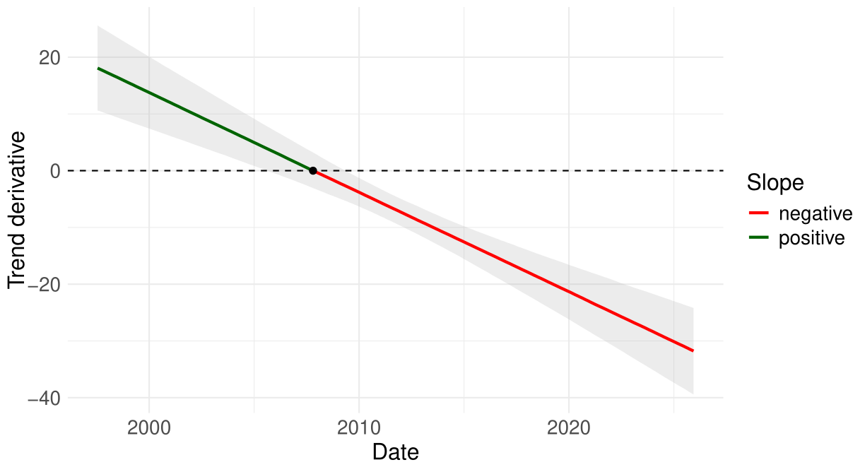
Observing Figure 1 we can see that The zero-crossing occurs around 2007-10-23 (median) with a 90% credible interval 2005-08-16 to 2009-05-07.

Discussion

Using the Harmonic regression model was vital for the removal of trend and seasonality components that make all the other models infeasible to use, since they do not work on un-stationary time series. The predisposition of a weekly trend was strongly supported by the findings of the fast Fourier analysis. We did find some high values at very low frequencies, but when calculating the $M$ for those values we got $M=n$ where $n$ is the number of datapoints in the dataset, so we ignored this frequency, since it does not make any sense.

We discovered that the data has no underlying MA process, since adding the MA part to our model made it much worse. In the end hierarchical AR model performed the best to the point that it was the only one used in our prediction ensamble.

The air quality seems to be increasing since 2007 which is a pleasant finding of our analysis.

https://github.com/fri-datascience/course_bs/blob/main/session_10_time_series/
data/no2.csv↩︎