Advanced Tracking
By Žan Pušenjak
Advanced Computer Vision Methods, FRI, University of Ljubljana
computer-vision object-tracking
Motion models and Kalman filter
First step to a functional tracker was the implementation of the Kalman filter. The algorithm depends on two parameters:
- denotes how much the filter trusts the dynamic model (models uncertainty).
- denotes how much the filter trusts the observation model (models uncertainty).
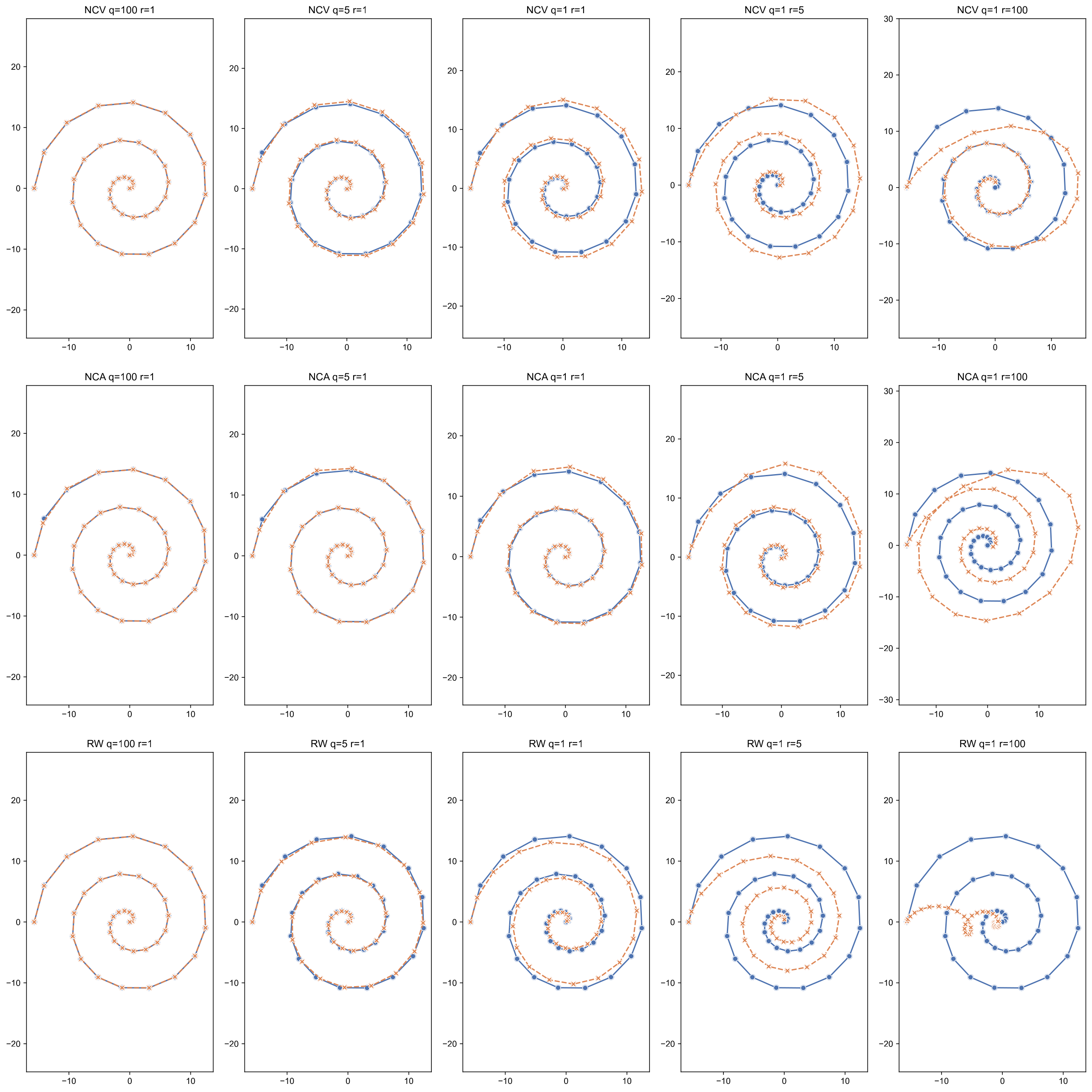
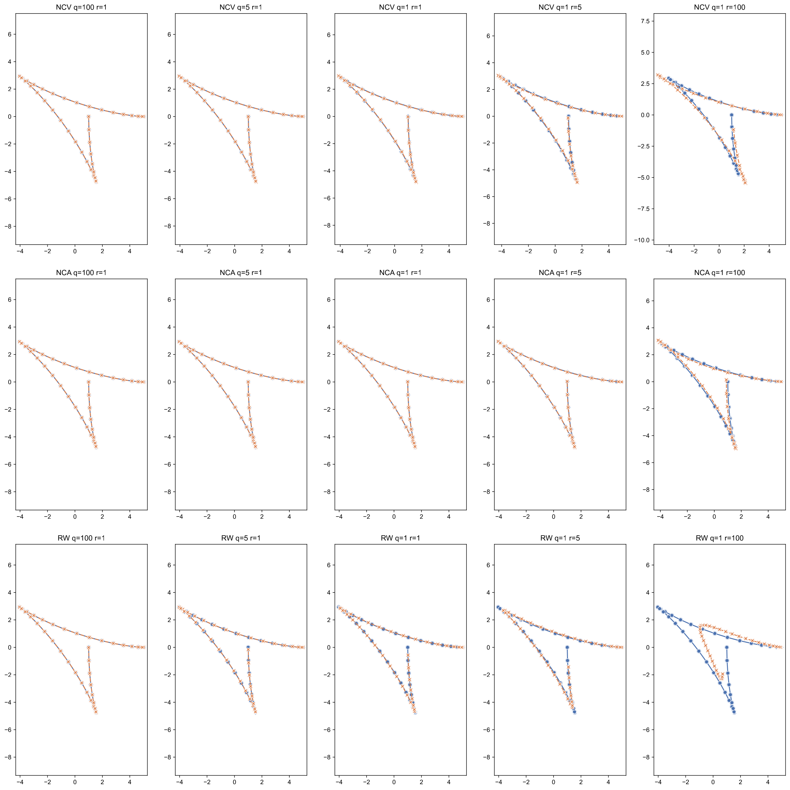
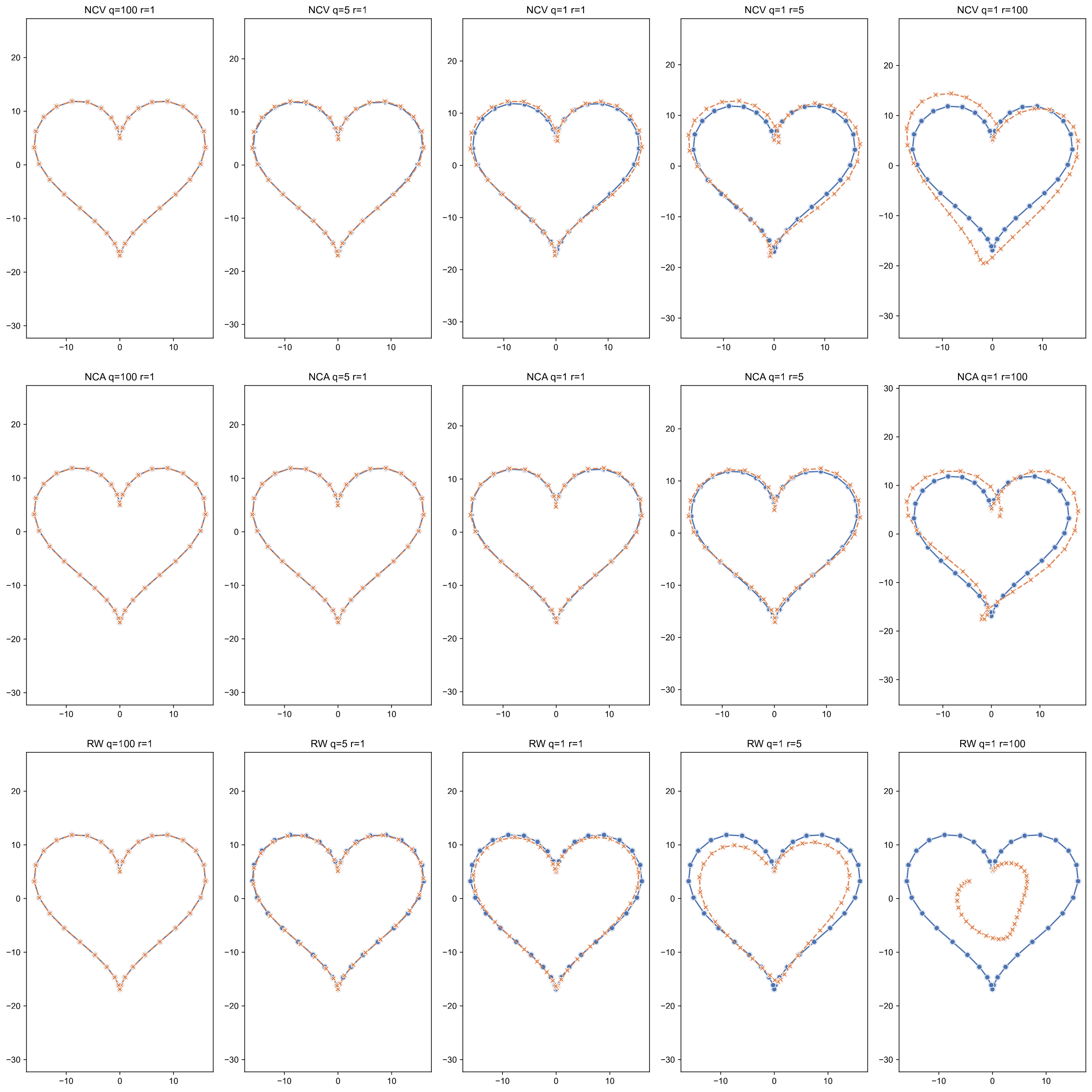
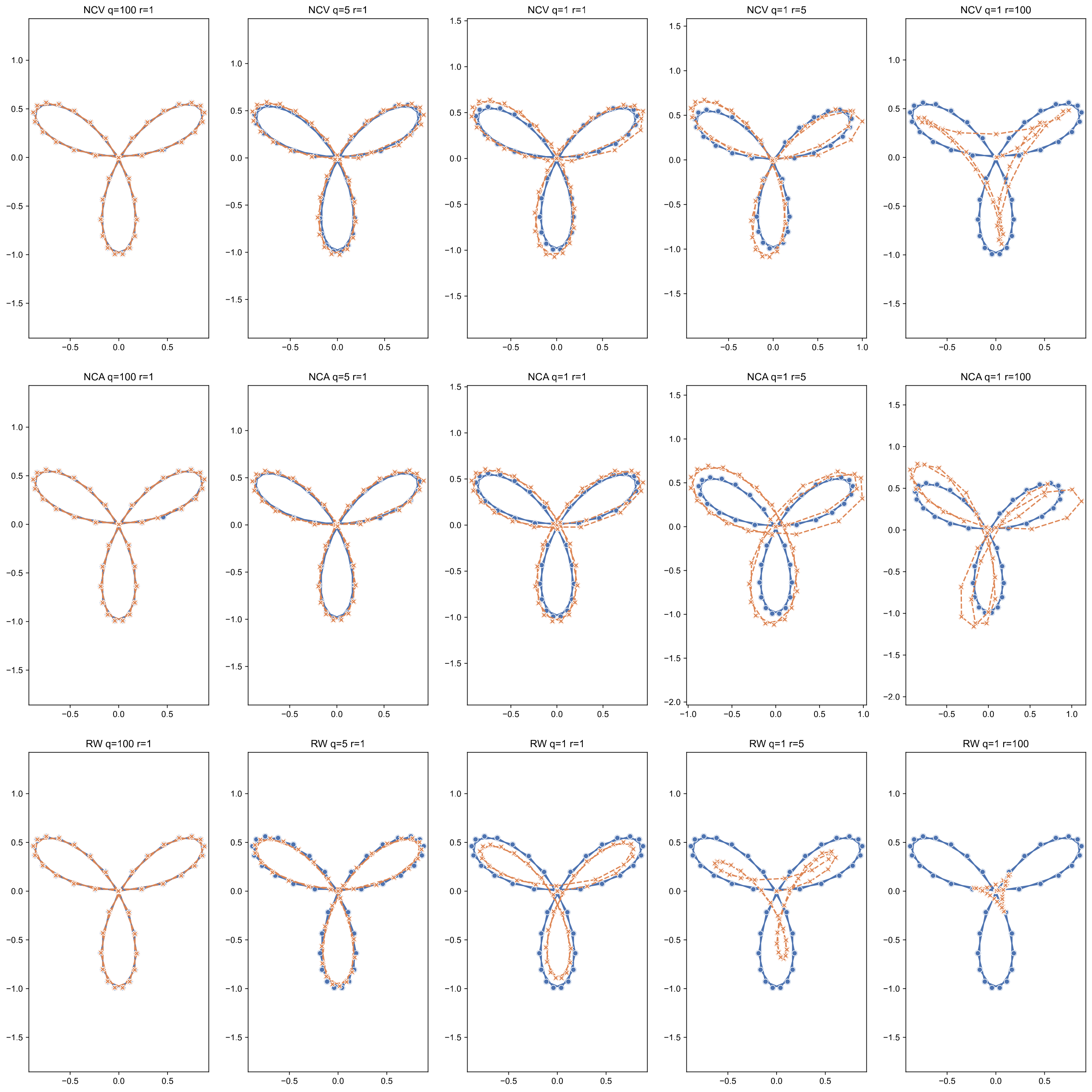
We implemented random Walk (RW), nearly-constant velocity (NCV), and nearly-constant acceleration (NCA) models and used them on different functions with various parameter combinations. The results can be observed in the appendix.
Observing the results we can clearly see, that a higher parameter matches the actual data completely (since the observations can be accurate), where lowering the and increasing the parameter increases the dynamic model influence and the difference between the ground truth and our predictions becomes increasingly larger.
Particle tracker
We implemented a particle tracker with different dynamic models and compared their performance. Further we tried to find the best set of tracker parameters.
We used the sequences from the VOT challenges1 more specifically the VOT14 set of challenges that include of twenty-five videos hand picked to test the reliability of trackers.
Implementation
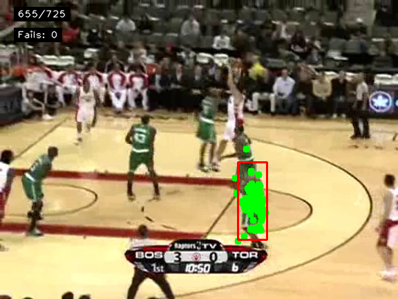
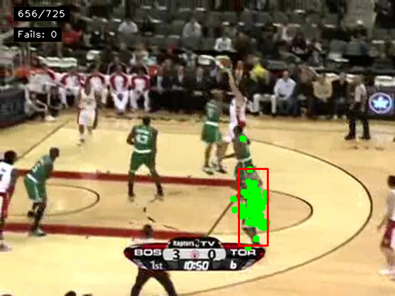
We implemented the particle tracker using the hellinger distance between color histograms and the following formula to calculate the likelihood. The parameter was set to since setting it any higher than that allowed particles far away to have a likelihood significant enough and the tracker would quickly drift if a similar object came close to the tracked one.
Based on the findings of previous assignments we used the following parameters:
- Since we used the Epanechnikov kernel2 we needed to determine its parameter.
- the number of bins for each color channel
We updated the template based on the parameter with the formula where is the template histogram and is the current found object histogram.
Surprisingly a higher than one used with the means-shift tracker showed better results.
Different models and parameter tuning
Lastly we used grid search to try and find the best possible set of parameters for our dataset. Because of computational reasons we used approximately five possible values for each of the parameters. Note that was fixed according to previous findings.
Additionally for RW and NCV models the was calculated based on the formula where correspond to the patch width and height, but the value was fixed at for the NCA model, since any greater value allowed the particles to move everywhere across the screen. The problem with the parameter is, that if the target is moving fast a higher is needed, but a higher value also means a less stable tracker, since the particles are much more uncertain.
Note that ecause the performance of the NCA model was not good, best score of 135 failures, we only plotted the RW and NCV model performance.
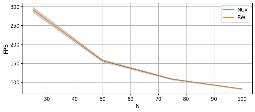
We can see that a higher number of particles yields a better performance overall, but is much more computationally expensive, so we have to make a decision about the resources used and our performance.
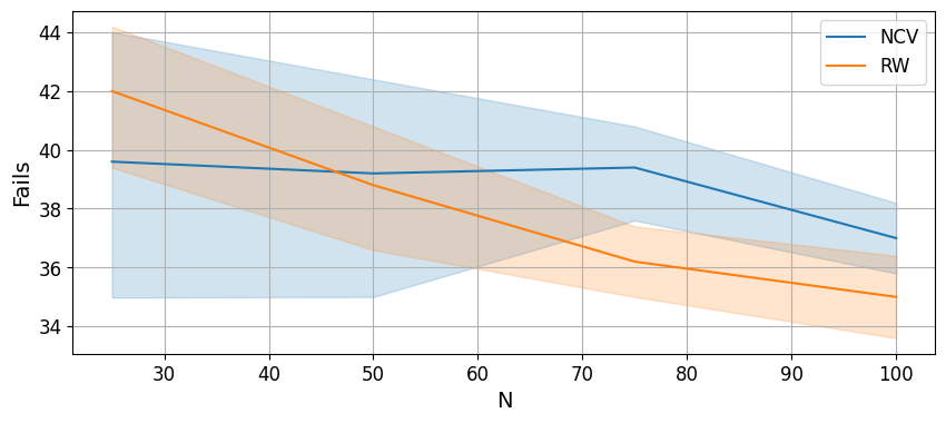
Also, the decision of the model is very important. Since almost no
entity moves with constant acceleration, the NCA model does not achieve
good results. If we look at the frames, we can observe, that the
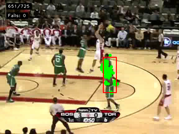
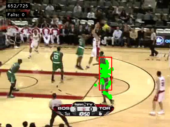
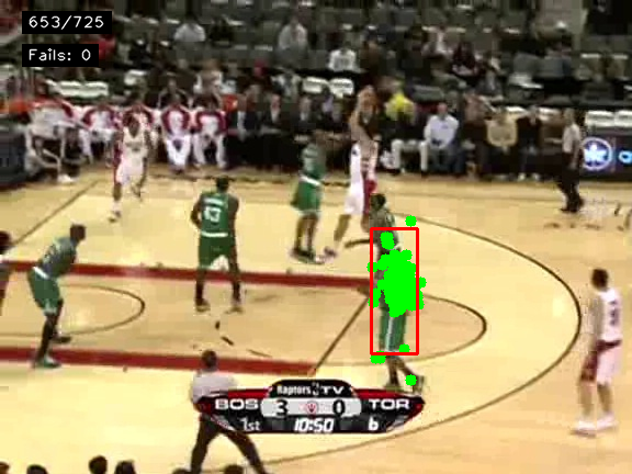
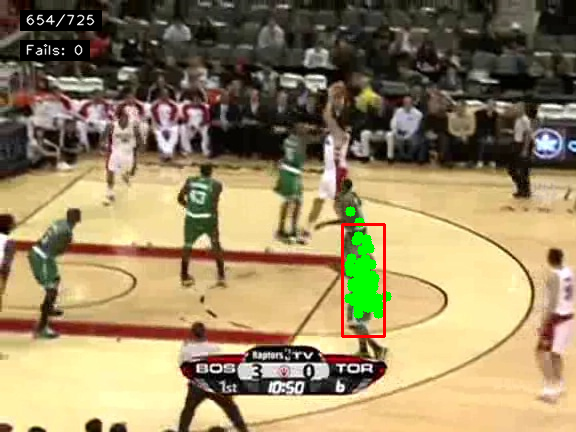
particles move around radically. Looking at the basketball
sequence1, when the player goes near another
player the tracker is able to drift off to the other player because the
particles are moving around so fiercely.
The best performance of 33 fails and 81 FPS was achieved with RW model with hundred particles. Note that the results varied, sometimes the NCV model achieved better results
Running the tracker with those parameters with the VOT evaluation toolkit3 were able to achieve an average overlap of , failures and an average FPS of .